
This is the third post in an eight part series that covers the fundamental theory of project management. This post focuses on Project Scheduling and is based on our online learning course Hands on Project Management Theory and Practice.
This post will discuss project time management focusing on scheduling. We will review the basic information used for project time management as well as models that represent this information to the project manager, including the Activity On Nodes (AON) network model and the Gantt chart. We will present the Critical Path analysis in both a deterministic (or certain) environment and in a stochastic (or uncertain) one. Additionally, we will see how Monte Carlo simulation can support scheduling decisions when uncertainty is present.
Project Time Management focuses on timely completion of:
- The project scope, which is the work content of the project
- The product scope, or the deliverables of the project.
For more information about Project Scope Management see the second post in this series.
In some projects timely completion is defined by a due date set by the stake holders. In other projects the goal is to finish the project as soon as possible. Yet in other projects timely completion means an effort to schedule the project so that its cost is minimized, or the profit generated by the project is maximized.
Due to the large variety of scheduling objectives it is important to understand the needs and expectations of the project stake holders with respect to time and to set the scheduling goals accordingly.
Before creating the project plan we should understand:
- The project target due date
- The penalty or bonus for finishing late or early.
In addition to the information on the project target due date and the associated bonus or penalty, information on the work content of the project is required for project time management. This information includes the list of tasks along with the precedence relations among them.
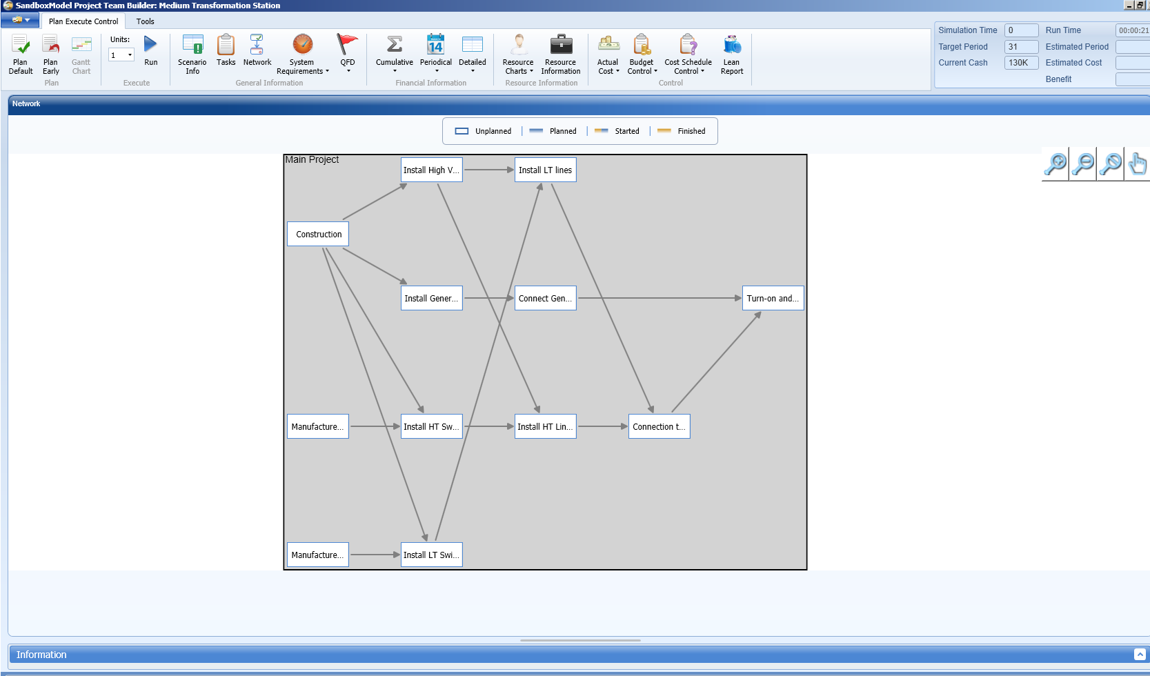
The presentation of project tasks and the precedence relations among them in the form of a table may not be the easiest presentation for analysis; therefore, other models for presentation of this data were developed.
A convenient way to present tasks and the precedence relations among them is the network model.
The third piece of information (in addition to the tasks and the precedence relations) required for scheduling is the duration of each task. At the planning phase the task duration is estimated or forecasted and therefore estimation errors are always present. If the estimate is accurate enough and the estimation error can be ignored, deterministic scheduling models can be used. The advantage of these models is their simplicity; the disadvantage is that uncertainty is ignored while we know that there is no way to forecast the exact duration of each task.
For each task or activity, we need to understand what is the expected duration range for each possible mode of execution.
If we go back to our radar project example, performing the task Transmitter Design in Technology A will have a duration of between 1-3 weeks while using Technology B, the more advanced technology, will have a duration of 2-5 weeks. Once we select the mode of execution for each activity we can get some estimates for the project duration.
A simple model for scheduling is the Gantt chart. In the Gantt chart each bar represents a project task and the duration of the tasks is represented by the length of the corresponding bar. The horizontal axis represents time since start of the project, also known as ARO – After Receiving Order. The leftmost point of the bar representing the task indicates its start time. The rightmost point of the bar indicates its finish time.
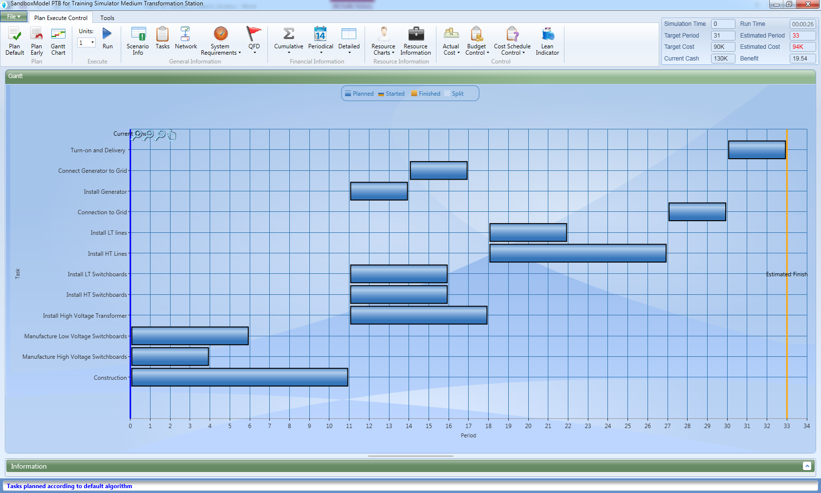
Due to precedence relations it is impossible to start all project tasks as soon as the project starts, as tasks having predecessors can only start once their predecessors are finished. The total project duration is determined by the longest sequence of tasks connecting the start of the project to its end. With a very small number of tasks the longest duration is easily identified. However, when the number of tasks increases, finding the longest duration is more difficult and special models are necessary to support decision making. One early model is the Critical Path Method or CPM.
The critical path of a project is defined as the longest sequence connecting the start of the project to its end. A special algorithm known as the Critical Path Method or CPM is used to find the critical tasks and the duration of the project.
The tasks on the critical path, also known as the critical tasks, comprise the longest sequence of tasks connecting the start of the project to its end. By definition, delay of critical tasks will cause a delay of the project. Non-critical tasks can be delayed by their slack, without delaying the project. This is illustrated in the late start Gantt chart.
In the late start Gantt chart critical activities’ start time is identical to the start time in the early start schedule. However, the start time of non-critical activities is delayed by as much as possible, without delaying the project. The amount of time a non-critical task can be delayed is known as the slack of that task.
The Gantt chart and the Critical Path Method are popular scheduling models, mainly because they are so easy to understand and to use. Their main weakness is that both ignore the impact of uncertainty. Since the project scope and the duration of tasks are estimates, they are subject to estimation errors. Therefore, there is a need for a model that will take uncertainty, and the resulting risk, into account.
Earlier models such as PERT, or Program Evaluation and Review Technique, were based on simplifying assumptions, mainly that it is good enough to focus on the critical path and to assume that its duration is normally distributed. These assumptions were made because the real stochastic scheduling problem is very hard to solve manually. The result was a very inaccurate analysis.
As the cost of computers decreased and their computational power increased, more accurate, computational extensive models were developed, to support project scheduling under uncertainty.
These models assume that the critical path may not be known for sure during the planning phase as the actual duration of each task is not known. Therefore, the best we can do is to use some measure of likelihood – how likely is each task to be on the critical path. This measure is known as the Criticality Index (CI) of project tasks.
The first step in stochastic scheduling is to replace the deterministic point estimate of task duration with a stochastic estimate, which takes uncertainty into account. A simple way to represent uncertainty in the duration of a project task is to estimate the shortest possible or optimistic duration, the longest possible or pessimistic duration and the most likely duration. These durations should be given to each possible alternative mode of execution of each task. The range of task duration is defined by the two extremes: the optimistic duration and the pessimistic duration. The most likely time tells us if the duration distribution is symmetrical or skewed. By using estimates for each mode, the project team can select the best project plan according to the scheduling requirements, while taking into account the other project constraints (cost, quality, risk, resources and so on).
With the three point estimate of task duration it is possible to simulate the project schedule by Monte Carlo simulation. The Monte Carlo simulation process is based on randomly generating the duration of each task from the relevant distribution and performing critical path analysis on the resulting task durations.
By repeating the process a large number of times the frequency that each task was on the critical path can be calculated. This frequency is an estimate of the task Criticality Index – the probability that the task is on the project critical path.
Each simulation run generates a critical path, and the duration distribution of these paths can be used to estimate the probability to finish the project by its due date, or any other date.
Although it is possible to use spreadsheets to perform the Monte Carlo simulation, special software tools exist that make it much easier and less time consuming.
The Monte Carlo simulation is a powerful tool that can help the project manager focus on risky tasks with high criticality index and to protect such tasks from delays. This process of identifying risks, mitigating those risks during the project planning phase and monitoring - controlling the risks during the project execution phase is key to project risk management. This will be discussed in the following posts in this series.